前言
前面的推文已经介绍过SSD算法,我觉得原理说的还算清楚了,但是一个算法不深入到代码去理解是完全不够的。因此本篇文章是在上篇SSD算法原理解析的基础上做的代码解析,解析SSD算法原理的推文的地址如下:https://mp.weixin.qq.com/s/lXqobT45S1wz-evc7KO5DA。今天要解析的SSD源码来自于github一个非常火的Pytorch实现,已经有3K+星,地址为:https://github.com/amdegroot/ssd.pytorch/
网络结构
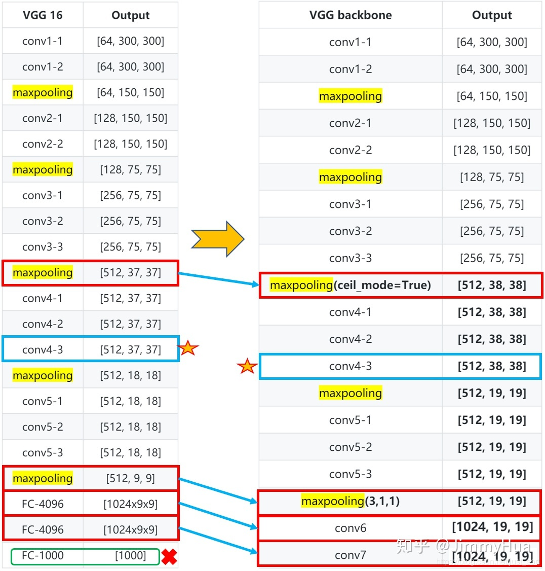
为了比较好的对应SSD的结构来看代码,我们首先放出SSD的网络结构,如下图所示:

可以看到原始的SSD网络是以VGG-16作Backbone(骨干网络)的。为了更加清晰看到相比于VGG16,SSD的网络使用了哪些变化,知乎上的一个帖子做了一个非常清晰的图,这里借用一下,原图地址为:https://zhuanlan.zhihu.com/p/79854543 。带有特征图维度信息的更清晰的骨干网络和VGG16的对比图如下:
源码解析
OK,现在我们就要开始从源码剖析SSD了 。主要弄清楚三个方面,网络结构的搭建,Anchor还有损失函数,就算是理解这个源码了。
网络搭建
从上面的图中我们可以清晰的看到在以VGG16做骨干网络时,在conv5后丢弃了CGG16中的全连接层改为了1024\times 3\times 3和1024\times1\times1的卷积层。其中conv4-1卷积层前面的maxpooling层的ceil_model=True,使得输出特征图长宽为38\times 38。还有conv5-3后面的一层maxpooling层参数为(kernelsize=3,stride=1,padding=1),不进行下采样。然后在fc7后面接上多尺度提取的另外4个卷积层就构成了完整的SSD网络。这里VGG16修改后的代码如下,来自ssd.py:
def vgg(cfg, i, batch_norm=False):
    layers = []
    in_channels = i
    for v in cfg:
        if v == 'M':
            layers += [nn.MaxPool2d(kernel_size=2, stride=2)]
        elif v == 'C':
            layers += [nn.MaxPool2d(kernel_size=2, stride=2, ceil_mode=True)]
        else:
            conv2d = nn.Conv2d(in_channels, v, kernel_size=3, padding=1)
            if batch_norm:
                layers += [conv2d, nn.BatchNorm2d(v), nn.ReLU(inplace=True)]
            else:
                layers += [conv2d, nn.ReLU(inplace=True)]
            in_channels = v
    pool5 = nn.MaxPool2d(kernel_size=3, stride=1, padding=1)
    conv6 = nn.Conv2d(512, 1024, kernel_size=3, padding=6, dilation=6)
    conv7 = nn.Conv2d(1024, 1024, kernel_size=1)
    layers += [pool5, conv6,
               nn.ReLU(inplace=True), conv7, nn.ReLU(inplace=True)]
    return layers
conv7就是我们上面图里面的fc7,特征维度是:[None,1024,19,19]。
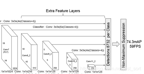
现在可以开始搭建SSD网络后面的多尺度提取网络了。也就是网络结构图中的Extra Feature Layers。我们从开篇的结构图中截取一下这一部分,方便我们对照代码。
实现的代码如下(同样来自ssd.py):
def add_extras(cfg, i, batch_norm=False):
    # Extra layers added to VGG for feature scaling
    layers = []
    in_channels = i
    flag = False #flag 用来控制 kernel_size= 1 or 3
    for k, v in enumerate(cfg):
        if in_channels != 'S':
            if v == 'S':
                layers += [nn.Conv2d(in_channels, cfg[k + 1],
                           kernel_size=(1, 3)[flag], stride=2, padding=1)]
            else:
                layers += [nn.Conv2d(in_channels, v, kernel_size=(1, 3)[flag])]
            flag = not flag
        in_channels = v
return layers
可以看到网络结构中除了魔改后的VGG16和Extra Layers还有6个横着的线,这代表的是对6个尺度的特征图进行卷积获得预测框的回归(loc)和类别(cls)信息,注意SSD将背景也看成类别了,所以对于VOC数据集类别数就是20+1=21。这部分的代码为:
def multibox(vgg, extra_layers, cfg, num_classes):
    loc_layers = []#多尺度分支的回归网络
    conf_layers = []#多尺度分支的分类网络
    # 第一部分,vgg 网络的 Conv2d-4_3(21层), Conv2d-7_1(-2层)
    vgg_source = [21, -2]
    for k, v in enumerate(vgg_source):
        # 回归 box*4(坐标)
        loc_layers += [nn.Conv2d(vgg[v].out_channels,
                                 cfg[k] * 4, kernel_size=3, padding=1)]
        # 置信度 box*(num_classes)
        conf_layers += [nn.Conv2d(vgg[v].out_channels,
                        cfg[k] * num_classes, kernel_size=3, padding=1)]
    # 第二部分,cfg从第三个开始作为box的个数,而且用于多尺度提取的网络分别为1,3,5,7层
    for k, v in enumerate(extra_layers[1::2], 2):
        loc_layers += [nn.Conv2d(v.out_channels, cfg[k]
                                 * 4, kernel_size=3, padding=1)]
        conf_layers += [nn.Conv2d(v.out_channels, cfg[k]
                                  * num_classes, kernel_size=3, padding=1)]
    return vgg, extra_layers, (loc_layers, conf_layers)
# 用下面的测试代码测试一下
if __name__  == "__main__":
    vgg, extra_layers, (l, c) = multibox(vgg(base['300'], 3),
                                         add_extras(extras['300'], 1024),
                                         [4, 6, 6, 6, 4, 4], 21)
    print(nn.Sequential(*l))
    print('---------------------------')
    print(nn.Sequential(*c))
'''
loc layers:
'''
Sequential(
  (0): Conv2d(512, 16, kernel_size=(3, 3), stride=(1, 1), padding=(1, 1))
  (1): Conv2d(1024, 24, kernel_size=(3, 3), stride=(1, 1), padding=(1, 1))
  (2): Conv2d(512, 24, kernel_size=(3, 3), stride=(1, 1), padding=(1, 1))
  (3): Conv2d(256, 24, kernel_size=(3, 3), stride=(1, 1), padding=(1, 1))
  (4): Conv2d(256, 16, kernel_size=(3, 3), stride=(1, 1), padding=(1, 1))
  (5): Conv2d(256, 16, kernel_size=(3, 3), stride=(1, 1), padding=(1, 1))
)
---------------------------
'''
conf layers:
'''
Sequential(
  (0): Conv2d(512, 84, kernel_size=(3, 3), stride=(1, 1), padding=(1, 1))
  (1): Conv2d(1024, 126, kernel_size=(3, 3), stride=(1, 1), padding=(1, 1))
  (2): Conv2d(512, 126, kernel_size=(3, 3), stride=(1, 1), padding=(1, 1))
  (3): Conv2d(256, 126, kernel_size=(3, 3), stride=(1, 1), padding=(1, 1))
  (4): Conv2d(256, 84, kernel_size=(3, 3), stride=(1, 1), padding=(1, 1))
  (5): Conv2d(256, 84, kernel_size=(3, 3), stride=(1, 1), padding=(1, 1))
)
Anchor生成(Prior_Box层)
这个在前面SSD的原理篇中讲过了,这里不妨再回忆一下,SSD从魔改后的VGG16的conv4_3开始一共使用了6个不同大小的特征图,大小分别为(38,28),(19,19),(10,10),(5,5),(3,3),(1,1),但每个特征图上设置的先验框(Anchor)的数量不同。先验框的设置包含尺度和长宽比两个方面。对于先验框的设置,公式如下:
s_k=s_{min}+\frac{s_{max}-s_{min}}{m-1}(k-1),k\in [1,m],其中M指的是特征图个数,这里为5,因为第一层conv4_3的Anchor是单独设置的,s_k代表先验框大小相对于特征图的比例,注意这里不是相对原图哦。最后,s_{min}和s_{max}表示比例的最小值和最大值,论文中分别取0.2和0.9。
对于第一个特征图,它的先验框尺度比例设置为s_{min}/2=0.1,则他的尺度为300\times 0.1=30,后面的特征图带入公式计算,并将其映射会原图300的大小可以得到,剩下的5个特征图的尺度s_k为{60,111,162,213,264}。所以综合起来,6个特征图的尺度s_k为{30,60,111,162,213,264}。有了Anchor的尺度,接下来设置Anchor的长宽,论文中长宽设置一般为a_r={1,2,3,\frac{1}{2},\frac{1}{3}},根据面积和长宽比可以得到先验框的宽度和高度: w_k^a=s_k\sqrt{a_r},h_k^a=s_k/\sqrt{a_r}。
这里有一些值得注意的点,如下:
- 上面的s_k是相对于原图的大小。
- 默认情况下,每个特征图除了上面5个比例的Anchor,还会设置一个尺度为s_k^{'}=\sqrt{s_ks_{k+1}}且a_r=1的先验框,这样每个特征图都设置了两个长宽比为1但大小不同的正方形先验框。最后一个特征图需要参考一下s_{m+1}=315来计算s_m。
- 在实现
conv4_3,conv10_2,conv11_2层时仅使用4个先验框,不使用长宽比为3,\frac{1}{3}的Anchor。 - 每个单元的先验框中心点分布在每个单元的中心,即: [\frac{i+0.5}{|f_k|},\frac{j+0.5}{|f_k|}],i,j\in[0,|f_k|],其中f_k是特征图的大小。
从Anchor的值来看,越前面的特征图Anchor的尺寸越小,也就是说对小目标的效果越好。先验框的总数为num_priors = 38x38x4+19x19x6+10x10x6+5x5x6+3x3x4+1x1x4=8732。
生成先验框的代码如下(来自layers/functions/prior_box.py)
class PriorBox(object):
    """Compute priorbox coordinates in center-offset form for each source
    feature map.
    """
    def __init__(self, cfg):
        super(PriorBox, self).__init__()
        self.image_size = cfg['min_dim']
        # number of priors for feature map location (either 4 or 6)
        self.num_priors = len(cfg['aspect_ratios'])
        self.variance = cfg['variance'] or [0.1]
        self.feature_maps = cfg['feature_maps']
        self.min_sizes = cfg['min_sizes']
        self.max_sizes = cfg['max_sizes']
        self.steps = cfg['steps']
        self.aspect_ratios = cfg['aspect_ratios']
        self.clip = cfg['clip']
        self.version = cfg['name']
        for v in self.variance:
            if v <= 0:
                raise ValueError('Variances must be greater than 0')

    def forward(self):
        mean = []
        # 遍历多尺度的 特征图: [38, 19, 10, 5, 3, 1]
        for k, f in enumerate(self.feature_maps):
            # 遍历每个像素
            for i, j in product(range(f), repeat=2):
                # k-th 层的feature map 大小
                f_k = self.image_size / self.steps[k]
                # # 每个框的中心坐标
                cx = (j + 0.5) / f_k
                cy = (i + 0.5) / f_k

                # aspect_ratio: 1 当 ratio==1的时候,会产生两个 box
                # r==1, size = s_k, 正方形
                s_k = self.min_sizes[k]/self.image_size
                mean += [cx, cy, s_k, s_k]

                # r==1, size = sqrt(s_k * s_(k+1)), 正方形
                # rel size: sqrt(s_k * s_(k+1))
                s_k_prime = sqrt(s_k * (self.max_sizes[k]/self.image_size))
                mean += [cx, cy, s_k_prime, s_k_prime]

                # 当 ratio != 1 的时候,产生的box为矩形
                for ar in self.aspect_ratios[k]:
                    mean += [cx, cy, s_k*sqrt(ar), s_k/sqrt(ar)]
                    mean += [cx, cy, s_k/sqrt(ar), s_k*sqrt(ar)]
        # 转化为 torch的Tensor
        output = torch.Tensor(mean).view(-1, 4)
        #归一化,把输出设置在 [0,1]
        if self.clip:
            output.clamp_(max=1, min=0)
return output
网络结构
结合了前面介绍的魔改后的VGG16,还有Extra Layers,还有生成Anchor的Priobox策略,我们可以写出SSD的整体结构如下(代码在ssd.py):
class SSD(nn.Module):
    """Single Shot Multibox Architecture
    The network is composed of a base VGG network followed by the
    added multibox conv layers.  Each multibox layer branches into
        1) conv2d for class conf scores
        2) conv2d for localization predictions
        3) associated priorbox layer to produce default bounding
           boxes specific to the layer's feature map size.
    See: https://arxiv.org/pdf/1512.02325.pdf for more details.
    Args:
        phase: (string) Can be "test" or "train"
        size: input image size
        base: VGG16 layers for input, size of either 300 or 500
        extras: extra layers that feed to multibox loc and conf layers
        head: "multibox head" consists of loc and conf conv layers
    """

    def __init__(self, phase, size, base, extras, head, num_classes):
        super(SSD, self).__init__()
        self.phase = phase
        self.num_classes = num_classes
        # 配置config
        self.cfg = (coco, voc)[num_classes == 21]
        # 初始化先验框
        self.priorbox = PriorBox(self.cfg)
        self.priors = Variable(self.priorbox.forward(), volatile=True)
        self.size = size

        # SSD network
        # backbone网络
        self.vgg = nn.ModuleList(base)
        # Layer learns to scale the l2 normalized features from conv4_3
        # conv4_3后面的网络,L2 正则化
        self.L2Norm = L2Norm(512, 20)
        self.extras = nn.ModuleList(extras)
        # 回归和分类网络
        self.loc = nn.ModuleList(head[0])
        self.conf = nn.ModuleList(head[1])

        if phase == 'test':
            self.softmax = nn.Softmax(dim=-1)
            self.detect = Detect(num_classes, 0, 200, 0.01, 0.45)

    def forward(self, x):
        """Applies network layers and ops on input image(s) x.
        Args:
            x: input image or batch of images. Shape: [batch,3,300,300].
        Return:
            Depending on phase:
            test:
                Variable(tensor) of output class label predictions,
                confidence score, and corresponding location predictions for
                each object detected. Shape: [batch,topk,7]
            train:
                list of concat outputs from:
                    1: confidence layers, Shape: [batch*num_priors,num_classes]
                    2: localization layers, Shape: [batch,num_priors*4]
                    3: priorbox layers, Shape: [2,num_priors*4]
        """
        sources = list()
        loc = list()
        conf = list()

        # apply vgg up to conv4_3 relu
        # vgg网络到conv4_3
        for k in range(23):
            x = self.vgg[k](x)
        # l2 正则化
        s = self.L2Norm(x)
        sources.append(s)

        # apply vgg up to fc7
        # conv4_3 到 fc
        for k in range(23, len(self.vgg)):
            x = self.vgg[k](x)
        sources.append(x)

        # apply extra layers and cache source layer outputs
        # extras 网络
        for k, v in enumerate(self.extras):
            x = F.relu(v(x), inplace=True)
            if k % 2 == 1:
                # 把需要进行多尺度的网络输出存入 sources
                sources.append(x)

        # apply multibox head to source layers
        # 多尺度回归和分类网络
        for (x, l, c) in zip(sources, self.loc, self.conf):
            loc.append(l(x).permute(0, 2, 3, 1).contiguous())
            conf.append(c(x).permute(0, 2, 3, 1).contiguous())

        loc = torch.cat([o.view(o.size(0), -1) for o in loc], 1)
        conf = torch.cat([o.view(o.size(0), -1) for o in conf], 1)
        if self.phase == "test":
            output = self.detect(
                loc.view(loc.size(0), -1, 4),                   # loc preds
                self.softmax(conf.view(conf.size(0), -1,
                             self.num_classes)),                # conf preds
                self.priors.type(type(x.data))                  # default boxes
            )
        else:
            output = (
                # loc的输出,size:(batch, 8732, 4)
                loc.view(loc.size(0), -1, 4),
                # conf的输出,size:(batch, 8732, 21)
                conf.view(conf.size(0), -1, self.num_classes),
                # 生成所有的候选框 size([8732, 4])
                self.priors
            )
        return output
    # 加载模型参数
    def load_weights(self, base_file):
        other, ext = os.path.splitext(base_file)
        if ext == '.pkl' or '.pth':
            print('Loading weights into state dict...')
            self.load_state_dict(torch.load(base_file,
                                 map_location=lambda storage, loc: storage))
            print('Finished!')
        else:
            print('Sorry only .pth and .pkl files supported.')
然后为了增加可读性,重新封装了一下,代码如下:
base = {
    '300': [64, 64, 'M', 128, 128, 'M', 256, 256, 256, 'C', 512, 512, 512, 'M',
            512, 512, 512],
    '512': [],
}
extras = {
    '300': [256, 'S', 512, 128, 'S', 256, 128, 256, 128, 256],
    '512': [],
}
mbox = {
    '300': [4, 6, 6, 6, 4, 4],  # number of boxes per feature map location
    '512': [],
}


def build_ssd(phase, size=300, num_classes=21):
    if phase != "test" and phase != "train":
        print("ERROR: Phase: " + phase + " not recognized")
        return
    if size != 300:
        print("ERROR: You specified size " + repr(size) + ". However, " +
              "currently only SSD300 (size=300) is supported!")
        return
    # 调用multibox,生成vgg,extras,head
    base_, extras_, head_ = multibox(vgg(base[str(size)], 3),
                                     add_extras(extras[str(size)], 1024),
                                     mbox[str(size)], num_classes)
    return SSD(phase, size, base_, extras_, head_, num_classes)
Loss解析
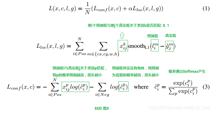
SSD的损失函数包含两个部分,一个是定位损失L_{loc},一个是分类损失L_{conf},整个损失函数表达如下:
L(x,c,l,g)=\frac{1}{N}(L_{conf}(x,c)+\alpha L_{loc}(x,l,g))
其中,N是先验框的正样本数量,c是类别置信度预测值,l是先验框对应的边界框预测值,g是ground truth的位置参数,x代表网络的预测值。对于位置损失,采用Smooth L1 Loss,位置信息都是encode之后的数值,后面会讲这个encode的过程。而对于分类损失,首先需要使用hard negtive mining将正负样本按照1:3 的比例把负样本抽样出来,抽样的方法是:针对所有batch的confidence,按照置信度误差进行降序排列,取出前top_k个负样本。损失函数可以用下图表示:
实现步骤
- Reshape所有batch中的conf,即代码中的
batch_conf = conf_data.view(-1, self.num_classes),方便后续排序。 - 置信度误差越大,实际上就是预测背景的置信度越小。
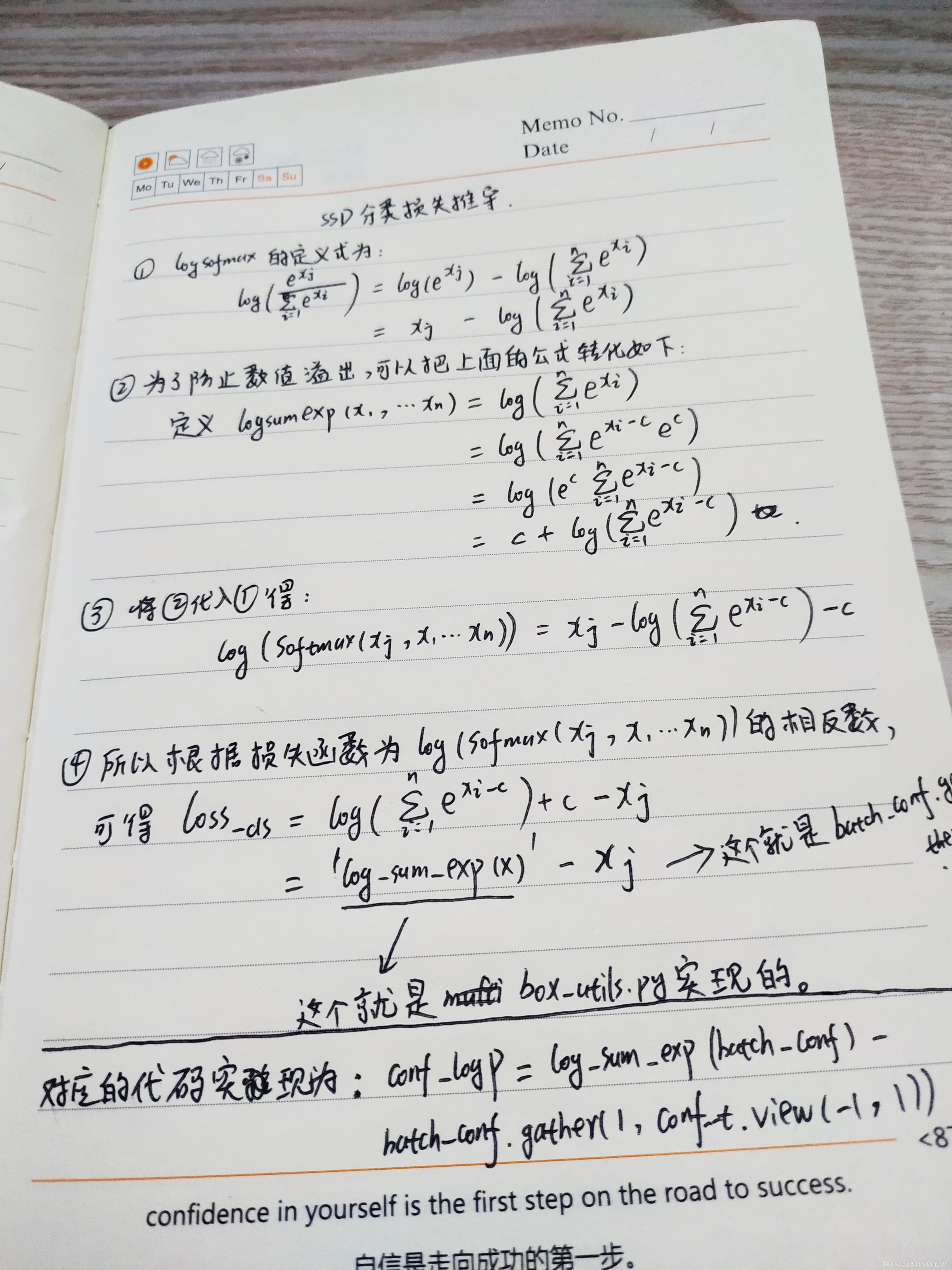
- 把所有conf进行
logsoftmax处理(均为负值),预测的置信度越小,则logsoftmax越小,取绝对值,则|logsoftmax|越大,降序排列-logsoftmax,取前top_k的负样本。 其中,log_sum_exp函数的代码如下:
def log_sum_exp(x):
    x_max = x.detach().max()
    return torch.log(torch.sum(torch.exp(x-x_max), 1, keepdim=True))+x_max
conf_logP函数如下:
conf_logP = log_sum_exp(batch_conf) - batch_conf.gather(1, conf_t.view(-1, 1))
这样计算的原因主要是为了增强logsoftmax损失的数值稳定性。放一张我的手推图:
损失函数完整代码实现,来自layers/modules/multibox_loss.py:
class MultiBoxLoss(nn.Module):
    """SSD Weighted Loss Function
    Compute Targets:
        1) Produce Confidence Target Indices by matching  ground truth boxes
           with (default) 'priorboxes' that have jaccard index > threshold parameter
           (default threshold: 0.5).
        2) Produce localization target by 'encoding' variance into offsets of ground
           truth boxes and their matched  'priorboxes'.
        3) Hard negative mining to filter the excessive number of negative examples
           that comes with using a large number of default bounding boxes.
           (default negative:positive ratio 3:1)
    Objective Loss:
        L(x,c,l,g) = (Lconf(x, c) + αLloc(x,l,g)) / N
        Where, Lconf is the CrossEntropy Loss and Lloc is the SmoothL1 Loss
        weighted by α which is set to 1 by cross val.
        Args:
            c: class confidences,
            l: predicted boxes,
            g: ground truth boxes
            N: number of matched default boxes
        See: https://arxiv.org/pdf/1512.02325.pdf for more details.
    """

    def __init__(self, num_classes, overlap_thresh, prior_for_matching,
                 bkg_label, neg_mining, neg_pos, neg_overlap, encode_target,
                 use_gpu=True):
        super(MultiBoxLoss, self).__init__()
        self.use_gpu = use_gpu
        self.num_classes = num_classes
        self.threshold = overlap_thresh
        self.background_label = bkg_label
        self.encode_target = encode_target
        self.use_prior_for_matching = prior_for_matching
        self.do_neg_mining = neg_mining
        self.negpos_ratio = neg_pos
        self.neg_overlap = neg_overlap
        self.variance = cfg['variance']

    def forward(self, predictions, targets):
        """Multibox Loss
        Args:
            predictions (tuple): A tuple containing loc preds, conf preds,
            and prior boxes from SSD net.
                conf shape: torch.size(batch_size,num_priors,num_classes)
                loc shape: torch.size(batch_size,num_priors,4)
                priors shape: torch.size(num_priors,4)
            targets (tensor): Ground truth boxes and labels for a batch,
                shape: [batch_size,num_objs,5] (last idx is the label).
        """
        loc_data, conf_data, priors = predictions
        num = loc_data.size(0)# batch_size
        priors = priors[:loc_data.size(1), :]
        num_priors = (priors.size(0)) # 先验框个数
        num_classes = self.num_classes #类别数

        # match priors (default boxes) and ground truth boxes
        # 获取匹配每个prior box的 ground truth
        # 创建 loc_t 和 conf_t 保存真实box的位置和类别
        loc_t = torch.Tensor(num, num_priors, 4)
        conf_t = torch.LongTensor(num, num_priors)
        for idx in range(num):
            truths = targets[idx][:, :-1].data #ground truth box信息
            labels = targets[idx][:, -1].data # ground truth conf信息
            defaults = priors.data # priors的 box 信息
            # 匹配 ground truth
            match(self.threshold, truths, defaults, self.variance, labels,
                  loc_t, conf_t, idx)
        if self.use_gpu:
            loc_t = loc_t.cuda()
            conf_t = conf_t.cuda()
        # wrap targets
        loc_t = Variable(loc_t, requires_grad=False)
        conf_t = Variable(conf_t, requires_grad=False)
        # 匹配中所有的正样本mask,shape[b,M]
        pos = conf_t > 0
        num_pos = pos.sum(dim=1, keepdim=True)
        # Localization Loss,使用 Smooth L1
        # shape[b,M]-->shape[b,M,4]
        pos_idx = pos.unsqueeze(pos.dim()).expand_as(loc_data)
        loc_p = loc_data[pos_idx].view(-1, 4) #预测的正样本box信息
        loc_t = loc_t[pos_idx].view(-1, 4) #真实的正样本box信息
        loss_l = F.smooth_l1_loss(loc_p, loc_t, size_average=False) #Smooth L1 损失

        '''
        Target;
            下面进行hard negative mining
        过程:
            1、 针对所有batch的conf,按照置信度误差(预测背景的置信度越小,误差越大)进行降序排列;
            2、 负样本的label全是背景,那么利用log softmax 计算出logP,
               logP越大,则背景概率越低,误差越大;
            3、 选取误差交大的top_k作为负样本,保证正负样本比例接近1:3;
        '''
        # Compute max conf across batch for hard negative mining
        # shape[b*M,num_classes]
        batch_conf = conf_data.view(-1, self.num_classes)
        # 使用logsoftmax,计算置信度,shape[b*M, 1]
        loss_c = log_sum_exp(batch_conf) - batch_conf.gather(1, conf_t.view(-1, 1))

        # Hard Negative Mining
        loss_c[pos] = 0  # 把正样本排除,剩下的就全是负样本,可以进行抽样
        loss_c = loss_c.view(num, -1)# shape[b, M]
        # 两次sort排序,能够得到每个元素在降序排列中的位置idx_rank
        _, loss_idx = loss_c.sort(1, descending=True)
        _, idx_rank = loss_idx.sort(1)
         # 抽取负样本
        # 每个batch中正样本的数目,shape[b,1]
        num_pos = pos.long().sum(1, keepdim=True)
        num_neg = torch.clamp(self.negpos_ratio*num_pos, max=pos.size(1)-1)
        # 抽取前top_k个负样本,shape[b, M]
        neg = idx_rank < num_neg.expand_as(idx_rank)

        # Confidence Loss Including Positive and Negative Examples
        # shape[b,M] --> shape[b,M,num_classes]
        pos_idx = pos.unsqueeze(2).expand_as(conf_data)
        neg_idx = neg.unsqueeze(2).expand_as(conf_data)
        # 提取出所有筛选好的正负样本(预测的和真实的)
        conf_p = conf_data[(pos_idx+neg_idx).gt(0)].view(-1, self.num_classes)
        targets_weighted = conf_t[(pos+neg).gt(0)]
        # 计算conf交叉熵
        loss_c = F.cross_entropy(conf_p, targets_weighted, size_average=False)

        # Sum of losses: L(x,c,l,g) = (Lconf(x, c) + αLloc(x,l,g)) / N
        # 正样本个数
        N = num_pos.data.sum()
        loss_l /= N
        loss_c /= N
        return loss_l, loss_c
先验框匹配策略
上面的代码中还有一个地方没讲到,就是match函数。这是SSD算法的先验框匹配函数。在训练时首先需要确定训练图片中的ground truth是由哪一个先验框来匹配,与之匹配的先验框所对应的边界框将负责预测它。SSD的先验框和ground truth匹配原则主要有2点。第一点是对于图片中的每个ground truth,找到和它IOU最大的先验框,该先验框与其匹配,这样可以保证每个ground truth一定与某个prior匹配。第二点是对于剩余的未匹配的先验框,若某个ground truth和它的IOU大于某个阈值(一般设为0.5),那么改prior和这个ground truth,剩下没有匹配上的先验框都是负样本(如果多个ground truth和某一个先验框的IOU均大于阈值,那么prior只与IOU最大的那个进行匹配)。代码实现如下,来自layers/box_utils.py:
def match(threshold, truths, priors, variances, labels, loc_t, conf_t, idx):
    """把和每个prior box 有最大的IOU的ground truth box进行匹配,
    同时,编码包围框,返回匹配的索引,对应的置信度和位置
    Args:
        threshold: IOU阈值,小于阈值设为背景
        truths: ground truth boxes, shape[N,4]
        priors: 先验框, shape[M,4]
        variances: prior的方差, list(float)
        labels: 图片的所有类别,shape[num_obj]
        loc_t: 用于填充encoded loc 目标张量
        conf_t: 用于填充encoded conf 目标张量
        idx: 现在的batch index
        The matched indices corresponding to 1)location and 2)confidence preds.
    """
    # jaccard index
    # 计算IOU
    overlaps = jaccard(
        truths,
        point_form(priors)
    )
    # (Bipartite Matching)
    # [1,num_objects] 和每个ground truth box 交集最大的 prior box
    best_prior_overlap, best_prior_idx = overlaps.max(1, keepdim=True)
    # [1,num_priors] 和每个prior box 交集最大的 ground truth box
    best_truth_overlap, best_truth_idx = overlaps.max(0, keepdim=True)
    best_truth_idx.squeeze_(0) #M
    best_truth_overlap.squeeze_(0) #M
    best_prior_idx.squeeze_(1) #N
    best_prior_overlap.squeeze_(1) #N
    # 保证每个ground truth box 与某一个prior box 匹配,固定值为 2 > threshold
    best_truth_overlap.index_fill_(0, best_prior_idx, 2)  # ensure best prior
    # TODO refactor: index  best_prior_idx with long tensor
    # ensure every gt matches with its prior of max overlap
    # 保证每一个ground truth 匹配它的都是具有最大IOU的prior
    # 根据 best_prior_dix 锁定 best_truth_idx里面的最大IOU prior
    for j in range(best_prior_idx.size(0)):
        best_truth_idx[best_prior_idx[j]] = j
    matches = truths[best_truth_idx]          # 提取出所有匹配的ground truth box, Shape: [M,4]
    conf = labels[best_truth_idx] + 1         # 提取出所有GT框的类别, Shape:[M]
    # 把 iou < threshold 的框类别设置为 bg,即为0
    conf[best_truth_overlap < threshold] = 0  # label as background
    # 编码包围框
    loc = encode(matches, priors, variances)
    # 保存匹配好的loc和conf到loc_t和conf_t中
    loc_t[idx] = loc    # [num_priors,4] encoded offsets to learn
    conf_t[idx] = conf  # [num_priors] top class label for each prior
位置坐标转换
我们看到上面出现了一个point_form函数,这是什么意思呢?这是因为目标框有2种表示方式:
- (x_{min},y_{min},x_{max},y_{max})
- (x,y,w,h)
这部分的代码在layers/box_utils.py下:
def point_form(boxes):
    """ Convert prior_boxes to (xmin, ymin, xmax, ymax)
   把 prior_box (cx, cy, w, h)转化为(xmin, ymin, xmax, ymax)
    """
    return torch.cat((boxes[:, :2] - boxes[:, 2:]/2,     # xmin, ymin
                     boxes[:, :2] + boxes[:, 2:]/2), 1)  # xmax, ymax


def center_size(boxes):
    """ Convert prior_boxes to (cx, cy, w, h)
    把 prior_box (xmin, ymin, xmax, ymax) 转化为 (cx, cy, w, h)
    """
    return torch.cat((boxes[:, 2:] + boxes[:, :2])/2,  # cx, cy
                            boxes[:, 2:] - boxes[:, :2], 1) # w, h
IOU计算
这部分比较简单,对于两个Box来讲,首先计算两个box左上角点坐标的最大值和右下角坐标的最小值,然后计算交集面积,最后把交集面积除以对应的并集面积。代码仍在layers/box_utils.py:
def intersect(box_a, box_b):
    """ We resize both tensors to [A,B,2] without new malloc:
    [A,2] -> [A,1,2] -> [A,B,2]
    [B,2] -> [1,B,2] -> [A,B,2]
    Then we compute the area of intersect between box_a and box_b.
    Args:
      box_a: (tensor) bounding boxes, Shape: [A,4].
      box_b: (tensor) bounding boxes, Shape: [B,4].
    Return:
      (tensor) intersection area, Shape: [A,B].
    """
    A = box_a.size(0)
    B = box_b.size(0)
     # 右下角,选出最小值
    max_xy = torch.min(box_a[:, 2:].unsqueeze(1).expand(A, B, 2),
                       box_b[:, 2:].unsqueeze(0).expand(A, B, 2))
    # 左上角,选出最大值
    min_xy = torch.max(box_a[:, :2].unsqueeze(1).expand(A, B, 2),
                       box_b[:, :2].unsqueeze(0).expand(A, B, 2))
    # 负数用0截断,为0代表交集为0
    inter = torch.clamp((max_xy - min_xy), min=0)
    return inter[:, :, 0] * inter[:, :, 1]


def jaccard(box_a, box_b):
    """Compute the jaccard overlap of two sets of boxes.  The jaccard overlap
    is simply the intersection over union of two boxes.  Here we operate on
    ground truth boxes and default boxes.
    E.g.:
        A ∩ B / A ∪ B = A ∩ B / (area(A) + area(B) - A ∩ B)
    Args:
        box_a: (tensor) Ground truth bounding boxes, Shape: [num_objects,4]
        box_b: (tensor) Prior boxes from priorbox layers, Shape: [num_priors,4]
    Return:
        jaccard overlap: (tensor) Shape: [box_a.size(0), box_b.size(0)]
    """
    inter = intersect(box_a, box_b)# A∩B
     # box_a和box_b的面积
    area_a = ((box_a[:, 2]-box_a[:, 0]) *
              (box_a[:, 3]-box_a[:, 1])).unsqueeze(1).expand_as(inter)  # [A,B]#(N,)
    area_b = ((box_b[:, 2]-box_b[:, 0]) *
              (box_b[:, 3]-box_b[:, 1])).unsqueeze(0).expand_as(inter)  # [A,B]#(M,)
    union = area_a + area_b - inter
    return inter / union  # [A,B]
L2标准化
VGG16的conv4_3特征图的大小为38\times 38,网络层靠前,方差比较大,需要加一个L2标准化,以保证和后面的检测层差异不是很大。L2标准化的公式如下:
\hat{x}=\frac{x}{||x||^2},其中x=(x_1...x_d)||x||_2=(\sum_{i=1}^d|x_i|^2)^{1/2}。同时,这里还要注意的是如果简单的对一个layer的输入进行L2标准化就会改变该层的规模,并且会减慢学习速度,因此这里引入了一个缩放系数\gamma_i
,对于每一个通道l2标准化后的结果为:
y_i=\gamma_i\hat{x_i},通常scale的值设10或者20,效果比较好。代码来自layers/modules/l2norm.py。
class L2Norm(nn.Module):
    '''
    conv4_3特征图大小38x38,网络层靠前,norm较大,需要加一个L2 Normalization,以保证和后面的检测层差异不是很大,具体可以参考: ParseNet。这个前面的推文里面有讲。
    '''
    def __init__(self, n_channels, scale):
        super(L2Norm, self).__init__()
        self.n_channels = n_channels
        self.gamma = scale or None
        self.eps = 1e-10
        # 将一个不可训练的类型Tensor转换成可以训练的类型 parameter
        self.weight = nn.Parameter(torch.Tensor(self.n_channels))
        self.reset_parameters()

    # 初始化参数
    def reset_parameters(self):
        nn.init.constant_(self.weight, self.gamma)

    def forward(self, x):
        # 计算x的2范数
        norm = x.pow(2).sum(dim=1, keepdim=True).sqrt() # shape[b,1,38,38]
        x = x / norm   # shape[b,512,38,38]

        # 扩展self.weight的维度为shape[1,512,1,1],然后参考公式计算
        out = self.weight[None,...,None,None] * x
        return out
位置信息编解码
上面提到了计算坐标损失的时候,坐标是encoding之后的,这是怎么回事呢?根据论文的描述,预测框和ground truth边界框存在一个转换关系,先定义一些变量:
- 先验框位置:d=(d^{cx},d^{cy},d^w,d^h)
- ground truth框位置:g=(g^{cx},g^{cy},g^w,g^h)
- variance是先验框的坐标方差。
然后编码的过程可以表示为:
\hat{g_j^{cx}}=(g_j^{cx}-d_i^{cx})/d_i^w/varicance[0] \hat{g_j^{cy}}=(g_j^{cy}-d_i^{cy})/d_i^h/varicance[1] \hat{g_j^w}=log(\frac{g_j^w}{d_i^w})/variance[2] \hat{g_j^h}=log(\frac{g_j^h}{d_i^h})/variance[3]
解码的过程可以表示为:
g_{predict}^{cx}=d^w*(variance[0]*l^{cx})+d^{cx} g_{predict}^{cy}=d^h*(variance[1]*l^{cy})+d^{cy} g_{predict}^w=d^wexp(vairance[2]*l^w) g_{predict}^h=d^hexp(vairance[3]*l^h)
这部分对应的代码在layers/box_utils.py里面:
def encode(matched, priors, variances):
    """Encode the variances from the priorbox layers into the ground truth boxes
    we have matched (based on jaccard overlap) with the prior boxes.
    Args:
        matched: (tensor) Coords of ground truth for each prior in point-form
            Shape: [num_priors, 4].
        priors: (tensor) Prior boxes in center-offset form
            Shape: [num_priors,4].
        variances: (list[float]) Variances of priorboxes
    Return:
        encoded boxes (tensor), Shape: [num_priors, 4]
    """

    # dist b/t match center and prior's center
    g_cxcy = (matched[:, :2] + matched[:, 2:])/2 - priors[:, :2]
    # encode variance
    g_cxcy /= (variances[0] * priors[:, 2:])
    # match wh / prior wh
    g_wh = (matched[:, 2:] - matched[:, :2]) / priors[:, 2:]
    g_wh = torch.log(g_wh) / variances[1]
    # return target for smooth_l1_loss
    return torch.cat([g_cxcy, g_wh], 1)  # [num_priors,4]


# Adapted from https://github.com/Hakuyume/chainer-ssd
def decode(loc, priors, variances):
    """Decode locations from predictions using priors to undo
    the encoding we did for offset regression at train time.
    Args:
        loc (tensor): location predictions for loc layers,
            Shape: [num_priors,4]
        priors (tensor): Prior boxes in center-offset form.
            Shape: [num_priors,4].
        variances: (list[float]) Variances of priorboxes
    Return:
        decoded bounding box predictions
    """

    boxes = torch.cat((
        priors[:, :2] + loc[:, :2] * variances[0] * priors[:, 2:],
        priors[:, 2:] * torch.exp(loc[:, 2:] * variances[1])), 1)
    boxes[:, :2] -= boxes[:, 2:] / 2
    boxes[:, 2:] += boxes[:, :2]
return boxes
后处理NMS
这部分我在上周的推文讲过原理了,这里不再赘述了。这里IOU阈值取了0.5。不了解原理可以去看一下我的那篇推文,也给了源码讲解,地址是:https://mp.weixin.qq.com/s/orYMdwZ1VwwIScPmIiq5iA 。这部分的代码也在layers/box_utils.py里面。就不再拿代码来赘述了。
检测函数
模型在测试的时候,需要把loc和conf输入到detect函数进行nms,然后给出结果。这部分的代码在layers/functions/detection.py里面,如下:
class Detect(Function):
    """At test time, Detect is the final layer of SSD.  Decode location preds,
    apply non-maximum suppression to location predictions based on conf
    scores and threshold to a top_k number of output predictions for both
    confidence score and locations.
    """
    def __init__(self, num_classes, bkg_label, top_k, conf_thresh, nms_thresh):
        self.num_classes = num_classes
        self.background_label = bkg_label
        self.top_k = top_k
        # Parameters used in nms.
        self.nms_thresh = nms_thresh
        if nms_thresh <= 0:
            raise ValueError('nms_threshold must be non negative.')
        self.conf_thresh = conf_thresh
        self.variance = cfg['variance']

    def forward(self, loc_data, conf_data, prior_data):
        """
        Args:
            loc_data: 预测出的loc张量,shape[b,M,4], eg:[b, 8732, 4]
            conf_data:预测出的置信度,shape[b,M,num_classes], eg:[b, 8732, 21]
            prior_data:先验框,shape[M,4], eg:[8732, 4]
        """
        num = loc_data.size(0)  # batch size
        num_priors = prior_data.size(0)
        output = torch.zeros(num, self.num_classes, self.top_k, 5)# 初始化输出
        conf_preds = conf_data.view(num, num_priors,
                                    self.num_classes).transpose(2, 1)

        # 解码loc的信息,变为正常的bboxes
        for i in range(num):
            # 解码loc
            decoded_boxes = decode(loc_data[i], prior_data, self.variance)
            # 拷贝每个batch内的conf,用于nms
            conf_scores = conf_preds[i].clone()
            # 遍历每一个类别
            for cl in range(1, self.num_classes):
                # 筛选掉 conf < conf_thresh 的conf
                c_mask = conf_scores[cl].gt(self.conf_thresh)
                scores = conf_scores[cl][c_mask]
                # 如果都被筛掉了,则跳入下一类
                if scores.size(0) == 0:
                    continue
                # 筛选掉 conf < conf_thresh 的框
                l_mask = c_mask.unsqueeze(1).expand_as(decoded_boxes)
                boxes = decoded_boxes[l_mask].view(-1, 4)
                # idx of highest scoring and non-overlapping boxes per class
                # nms
                ids, count = nms(boxes, scores, self.nms_thresh, self.top_k)
                # nms 后得到的输出拼接
                output[i, cl, :count] = \
                    torch.cat((scores[ids[:count]].unsqueeze(1),
                               boxes[ids[:count]]), 1)
        flt = output.contiguous().view(num, -1, 5)
        _, idx = flt[:, :, 0].sort(1, descending=True)
        _, rank = idx.sort(1)
        flt[(rank < self.top_k).unsqueeze(-1).expand_as(flt)].fill_(0)
    return output
后记
SSD的核心代码解析大概就到这里了,我觉得这个过程算法还算比较清晰了,不过SSD能够表现较好的原因还和它的多种有效的数据增强方式有关,之后我们有机会再来解析一下他的数据增强策略。本文写作的目录参考了知乎https://zhuanlan.zhihu.com/p/79854543,看代码和写作以及理解一些细节大概花了一周时间,看到这里的同学不妨给我点个赞吧。
欢迎关注我的微信公众号GiantPandaCV,期待和你一起交流机器学习,深度学习,图像算法,优化技术,比赛及日常生活等。
本文总阅读量次