【Attention Transfer】paying more attention to attention¶

论文名：Paying more attention to attention: improving the performance of convolutional neural networks via Attention Transfer

接受：ICLR2017

解决问题：为了提升学生网络的性能。

解决方案：提出了transferring attention, 目标是训练出的学生模型不仅预测精度更高，而且还需要让他们的特征图与教师网络的特征图相似。

介绍¶

有关注意力的一个假设：

非注意力视觉过程可以用于感知整体场景，聚合高层信息，可以用于控制注意过程，引导到场景的某个部分。
但是不同的视觉系统的观察角度可能不相同，如何利用注意力信息来提升性能是一个值得研究的问题。
更具体来讲如何使用教师网络来提升其他学生网络的性能。

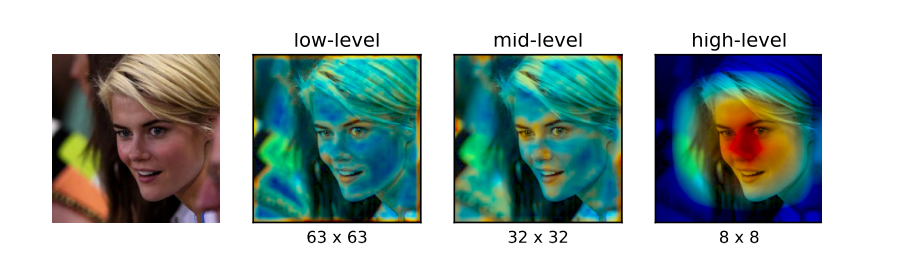
注意力选择方面：AT选择使用空间注意力图，空间注意力图具有更高的可解释性。同时网络不同阶段的特征图拥有者捕获底层、中层、高层的表征信息。具体来说可以划分为：

activation-based spatial attention maps
gradient-based spatial attention maps

本文具体贡献：

提出使用attention作为迁移知识的特殊机制。
提出同时使用activation-based 和 gradient-based spatial attention maps
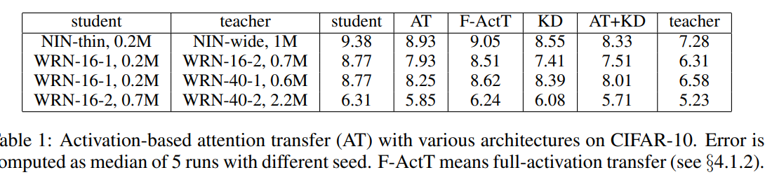
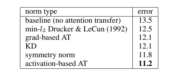
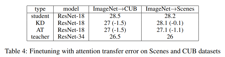
实验证明可以有一定的提升，并且要比full-activation transfer性能更好，可以与KD相结合。

Attention Transfer¶

1. Activation-based Attention Transfer¶

使用一个转换，可以将三维特征图转化为一维的HxW的空间特征图

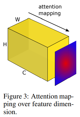
$\mathcal{F}: R^{C \times H \times W} \rightarrow R^{H \times W}$

具体来说有几种实现方案：

求和： $F_{\mathrm{sum}}(A)=\sum_{i=1}^{C}\left|A_{i}\right|$
求P范数（p>1）： $F_{\text {sum }}^{p}(A)=\sum_{i=1}^{C}\left|A_{i}\right|^{p}$
求max P范数（p>1）: $F_{\max }^{p}(A)=\max _{i=1, C}\left|A_{i}\right|^{p}$

对activation map进行可视化：

那么在哪个地方施加注意力？对应阶段！

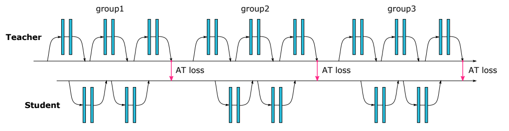
具体计算公式：

$\mathcal{L}_{A T}=\mathcal{L}\left(\mathbf{W}_{S}, x\right)+\frac{\beta}{2} \sum_{j \in \mathcal{I}}\left\|\frac{Q_{S}^{j}}{\left\|Q_{S}^{j}\right\|_{2}}-\frac{Q_{T}^{j}}{\left\|Q_{T}^{j}\right\|_{2}}\right\|_{p}$

L(ws,x)是交叉熵公式，Q代表对应层的attention maps，第二项使用的是L2范数。

ps：如果空间特征图尺寸不匹配，会采用插值的方式保持一致。所以这启发我们可以使用通道注意力，虽然可解释性没那么强，但是扩展性好。

2. Gradient-based Attention Transfer¶

将注意力定义为梯度，也即输入，可以被视为input sensitivity map。按照以下公式定义教师网络和学生网络梯度：

$J_{S}=\frac{\partial}{\partial x} \mathcal{L}\left(\mathbf{W}_{\mathbf{S}}, x\right), J_{T}=\frac{\partial}{\partial x} \mathcal{L}\left(\mathbf{W}_{\mathbf{T}}, x\right)$

为了让两者梯度尽可能相似，使用以下loss:

$\mathcal{L}_{A T}\left(\mathbf{W}_{\mathbf{S}}, \mathbf{W}_{\mathbf{T}}, x\right)=\mathcal{L}\left(\mathbf{W}_{\mathbf{S}}, x\right)+\frac{\beta}{2}\left\|J_{S}-J_{T}\right\|_{2}$

那么对应的梯度计算如下：

$\frac{\partial}{\partial \mathbf{W}_{\mathbf{S}}} \mathcal{L}_{A T}=\frac{\partial}{\partial \mathbf{W}_{\mathbf{S}}} \mathcal{L}\left(\mathbf{W}_{\mathbf{S}}, x\right)+\beta\left(J_{S}-J_{T}\right) \frac{\partial^{2}}{\partial \mathbf{W}_{\mathbf{S}} \partial x} \mathcal{L}\left(\mathbf{W}_{\mathbf{S}}, x\right)$

实验部分¶

实现¶

网络forward实现：o是最终embedding，g0,g1,g2代表三个stage的输出结果。

  def f(input, params, mode, base=''):
      x = F.conv2d(input, params[f'{base}conv0'], padding=1)
      g0 = group(x, params, f'{base}group0', mode, 1)
      g1 = group(g0, params, f'{base}group1', mode, 2)
      g2 = group(g1, params, f'{base}group2', mode, 2)
      o = F.relu(utils.batch_norm(g2, params, f'{base}bn', mode))
      o = F.avg_pool2d(o, 8, 1, 0)
      o = o.view(o.size(0), -1)
      o = F.linear(o, params[f'{base}fc.weight'], params[f'{base}fc.bias'])
      return o, (g0, g1, g2)

KD hinton实现：

def distillation(y, teacher_scores, labels, T, alpha):
    p = F.log_softmax(y/T, dim=1)
    q = F.softmax(teacher_scores/T, dim=1)
    l_kl = F.kl_div(p, q, size_average=False) * (T**2) / y.shape[0]
    l_ce = F.cross_entropy(y, labels)
    return l_kl * alpha + l_ce * (1. - alpha)

feature map l2 loss实现：

def at_loss(x, y):
    return (at(x) - at(y)).pow(2).mean()

整体loss实现：

y_s, y_t, loss_groups = utils.data_parallel(f, inputs, params, sample[2], range(opt.ngpu))
loss_groups = [v.sum() for v in loss_groups]
return utils.distillation(y_s, y_t, targets, opt.temperature, opt.alpha) + opt.beta * sum(loss_groups), y_s

本文总阅读量次